2025-02-28 Weekly Notes

28 February 2025

This week I focused mostly on checking why I had some empty rows in the estimation of the canopy cover and the tree count from the Vegetation Object Model. After investigating the code, I found that the issue was behind a try/except clause that was masking corrupted files. Now, this was the intended behaviour originally, as some files can’t be read, however, because the data processing is done at the geographic statistical level (read ONS), and the VOM tiles come in 5x5 km files (following GB National Grid), even when one file can’t be read, the other ones wouldn’t be processed either. With the new small correction, only the corrupted files are not processed and the rest of the files are processed as intended. So from the 5402 tiles, only 26 can’t be read.

In addition to this, I wanted to reduce the over segmentation of trees from the VOM, because I was getting way more tree points than there actually are (at least visually), which leads to an overestimation of the number of trees. To do so, two changes were made thanks to chatGPT 🙃:

Increase the size of the matrix for focal smoothing for each raster file
Turn the Local Maxima Filter (LMF) function into a Gaussian distribution (inspired by Gaussian heatmap work I saw in BIOSPACE25)

With this change, I estimated a reduction of ~60% in the number of trees, which doesn’t mean that there are more False Negatives, it just means that trees are grouped into fewer instances and tend to be bigger (particularly in clustered areas). Unfortunately (or fortunately, depending on who you ask), the code is written in R through the lidR package, so processing takes a bit longer. In addition, I found out that when you discard changes made in VS Code by Copilot, it will bring back the latest comitted changes, which is a bit annoying, and for that reason I had to repeat the entire run twice, as it had executed the code without the aforementioned changes. Apparently R makes extensive use of the /tmp folder which caused some issues in Kinabalu, as quickly pointed out by Michael.

Another optimisation step that I could implement in the code was to reduce the number of iterations to get the number of trees in a 100 m radius around each building. As mentioned before, the processing is done at a geographic level which for me initially was at the LSOA level (roughly equivalent to neighbourhood), the smallest possible, however the VOM tiles and the subsequent tree vector layers span 25 km2, which covers more than one LSOA, so I was reading the same file multiple times when processing for different LSOAs. To avoid this, I am now using the LAD level (roughly equivalent to city), the next one in size, which means that I am reducing the number of iterations from 32k to 300 but I am processing more tree tiles per iteration in Sedona. When I ran this the first time it took 11 days, but I’m guessing this one shouldn’t take more than 3 days.

In other news, I got rejected from the IPCC Chapter Scientist application I sent a couple of weeks ago 😕, but I got a follow up email to fill in a form for a visitng student position in one of the big tech companies 🤓 for the summer, which doesn’t mean that I passed a filter round, it just means that they are collecting more info than there is in the CV.

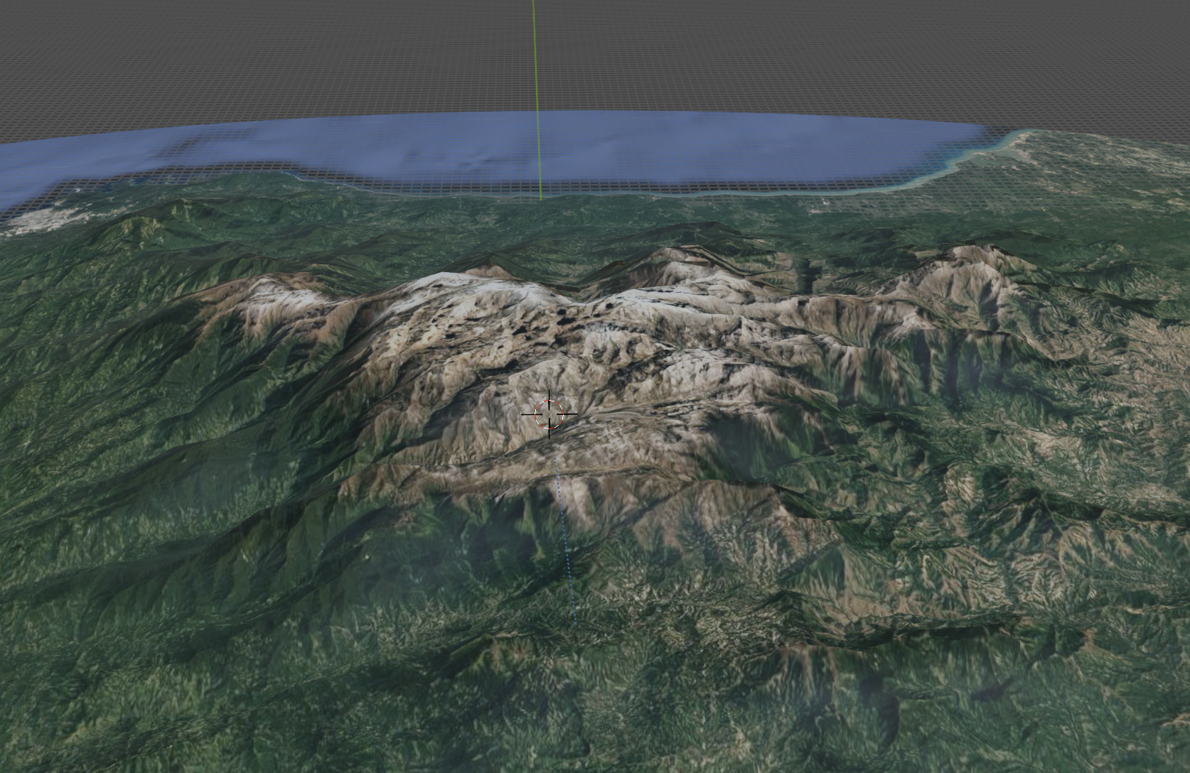
Finally, I also attended a workshop organised by London Data Visualisation on how to make 3D maps in Blender. It was taught by Julian Hoffman Anton in the Canva HQ in London. It was pretty cool to see what you can do when you combine GIS data with Blender. I’m not sure if I will use it in the future, but it was a nice experience to see how you can make 3D maps with minimal coding and a lot of creativity. The picture below is my attempt at trying to visualize the tallest coastal mountain in the world (Sierra Nevada de Santa Marta) using Google imagery and open topography data.