
Code
%load_ext autoreload
%autoreload 2
import sys
sys.path.append('../src')%load_ext autoreload
%autoreload 2
import sys
sys.path.append('../src')This notebook presents a minimal example of how to create a deep learning model for classification of LCZ classes using Tessera embeddings and a couple of labels for Nairobi. It uses Torchgeo to handle dataloaders and Sadiq’s U-net architecture for solar farm detection with a couple of tweaks on the loss because most of the ROI is not labeled.
import glob
import warnings
warnings.filterwarnings('ignore')

import numpy as np
import geopandas as gpd
import rasterio
import rasterio.windows
from rasterio.merge import merge
from shapely.geometry import box as shapely_box

import torch
import torch.nn as nn
import torch.optim as optim
from torch.utils.data import Dataset, DataLoader
import matplotlib.pyplot as plt

from train_unet import UNet, MulticlassDiceLossTIF_DIR = '/maps/acz25/phd-thesis-data/input/Embeddings_test/GeoTessera/2017/'
LABEL_PATH = '/maps/acz25/phd-thesis-data/input/So2Sat-LCZ42/v4/patches_reference_Nairobi.gpkg'
LABEL_COL = 'LCZ_class'
IN_CHANNELS = 128
NUM_CLASSES = 17
PATCH_SIZE = 32 # pixels (320 m at 10 m/px)
BATCH_SIZE = 16
EPOCHS = 5
DICE_WEIGHT = 0.5
DEVICE = torch.device('cuda' if torch.cuda.is_available() else 'cpu')
print('device:', DEVICE)device: cudafrom matplotlib.colors import ListedColormap, BoundaryNorm
from matplotlib.patches import Patch
lcz_dict = {
1: {"name": "Compact High-Rise", "alt_code": "1", "color": "#8c0000"},
2: {"name": "Compact Mid-Rise", "alt_code": "2", "color": "#d10000"},
3: {"name": "Compact Low-Rise", "alt_code": "3", "color": "#ff0000"},
4: {"name": "Open High-Rise", "alt_code": "4", "color": "#bf4d00"},
5: {"name": "Open Mid-Rise", "alt_code": "5", "color": "#ff6600"},
6: {"name": "Open Low-Rise", "alt_code": "6", "color": "#ff9955"},
7: {"name": "Lightweight Low-Rise", "alt_code": "7", "color": "#faee05"},
8: {"name": "Large Low-Rise", "alt_code": "8", "color": "#bcbcbc"},
9: {"name": "Sparsely Built", "alt_code": "9", "color": "#ffccaa"},
10: {"name": "Heavy Industry", "alt_code": "10", "color": "#555555"},
11: {"name": "Dense Trees", "alt_code": "A", "color": "#006a00"},
12: {"name": "Scattered Trees", "alt_code": "B", "color": "#00aa00"},
13: {"name": "Bush, Scrub", "alt_code": "C", "color": "#648525"},
14: {"name": "Low Plants", "alt_code": "D", "color": "#b9db79"},
15: {"name": "Bare Rock or Paved", "alt_code": "E", "color": "#000000"},
16: {"name": "Bare Soil or Sand", "alt_code": "F", "color": "#fbf7ae"},
17: {"name": "Water", "alt_code": "G", "color": "#6a6aff"},
}
# Colormap: index 0 = LCZ 1, ..., index 16 = LCZ 17
lcz_colors = [lcz_dict[c]['color'] for c in range(1, 18)]
lcz_cmap = ListedColormap(lcz_colors, name='lcz')
lcz_norm = BoundaryNorm(boundaries=np.arange(-0.5, 17.5, 1), ncolors=17)
def lcz_legend_handles():
return [
Patch(facecolor=lcz_dict[c]['color'],
label=f"LCZ {lcz_dict[c]['alt_code']}: {lcz_dict[c]['name']}")
for c in range(1, 18)
]Read every TIF’s bounding box into a GeoDataFrame.
This lets us quickly look up which tiles cover any given polygon.
tif_paths = sorted(glob.glob(TIF_DIR + '*.tif'))
print(f'{len(tif_paths)} TIF tiles')

# Read CRS from the first tile
with rasterio.open(tif_paths[0]) as src:
    TIF_CRS = src.crs
    print('CRS:', TIF_CRS)
    print('resolution:', src.res)
    print('bands:', src.count)

records = []
for p in tif_paths:
    with rasterio.open(p) as src:
        records.append({'path': p, 'geometry': shapely_box(*src.bounds)})

tif_index = gpd.GeoDataFrame(records, crs=TIF_CRS)
tif_index.plot(figsize=(6, 6), edgecolor='steelblue', facecolor='none')
plt.title('TIF tile coverage')
plt.show()
56 TIF tiles
CRS: EPSG:32737
resolution: (10.0, 10.0)
bands: 128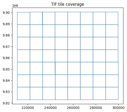
So2Sat patches are 320 m × 320 m polygons (32 px at 10 m/px), each with a single LCZ class.
The polygons overlap — adjacent patches share boundary pixels.
We handle this by treating each polygon as an independent training sample,
so overlaps never appear within a single patch.
gdf_wgs84 = gpd.read_file(LABEL_PATH)
gdf = gdf_wgs84.to_crs(TIF_CRS)
print(f'Polygons: {len(gdf)}  |  CRS: {gdf.crs}')
print(f'LCZ range: {gdf[LABEL_COL].min()} - {gdf[LABEL_COL].max()}')

fig, axes = plt.subplots(1, 2, figsize=(14, 5))

# Map: colour each polygon by its exact LCZ hex colour
gdf.plot(color=gdf[LABEL_COL].map(lambda c: lcz_dict[c]['color']), ax=axes[0], alpha=0.9)
axes[0].set_title('So2Sat LCZ patches (Nairobi)')
axes[0].set_xlabel('Easting (m)')
axes[0].set_ylabel('Northing (m)')

# Bar chart: one bar per class, coloured with LCZ palette
counts = gdf[LABEL_COL].value_counts().sort_index()
bar_colors = [lcz_dict[c]['color'] for c in counts.index]
counts.plot.bar(ax=axes[1], color=bar_colors, edgecolor='grey', linewidth=0.4)
axes[1].set_title('Class distribution')
axes[1].set_xlabel('LCZ class')
axes[1].set_ylabel('Count')
axes[1].set_xticklabels(
    [f"{c}\n{lcz_dict[c]['alt_code']}" for c in counts.index], rotation=0
)

# Shared legend
fig.legend(handles=lcz_legend_handles(), fontsize=9, ncol=6,
           loc='lower center', bbox_to_anchor=(0.5, -0.12), framealpha=0.8)

plt.tight_layout()
plt.show()
Polygons: 4828 | CRS: PROJCS["WGS 84 / UTM zone 37S",GEOGCS["WGS 84",DATUM["WGS_1984",SPHEROID["WGS 84",6378137,298.257223563,AUTHORITY["EPSG","7030"]],AUTHORITY["EPSG","6326"]],PRIMEM["Greenwich",0,AUTHORITY["EPSG","8901"]],UNIT["degree",0.0174532925199433,AUTHORITY["EPSG","9122"]],AUTHORITY["EPSG","4326"]],PROJECTION["Transverse_Mercator"],PARAMETER["latitude_of_origin",0],PARAMETER["central_meridian",39],PARAMETER["scale_factor",0.9996],PARAMETER["false_easting",500000],PARAMETER["false_northing",10000000],UNIT["metre",1,AUTHORITY["EPSG","9001"]],AXIS["Easting",EAST],AXIS["Northing",NORTH],AUTHORITY["EPSG","32737"]]
LCZ range: 1 - 17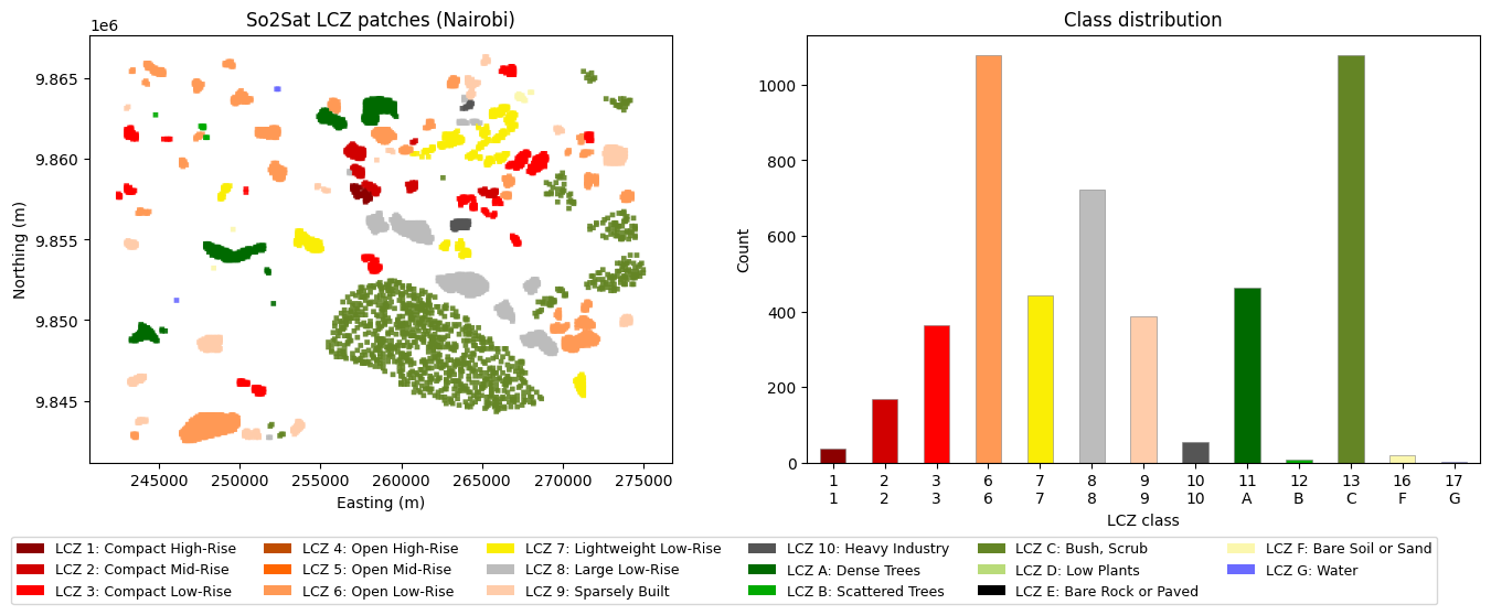
Each item in the dataset is one So2Sat polygon: - image: (128, 32, 32) Tessera embedding cropped to the polygon bounds
- mask: (32, 32) filled with the polygon’s LCZ class (0-indexed)
When a polygon crosses multiple TIF tiles, rasterio.merge mosaics them first.
Overlapping polygons are not a problem — each is an independent sample.
class PolygonPatchDataset(Dataset):
    """One sample per So2Sat polygon: (128, 32, 32) embedding + (32, 32) class mask."""

    def __init__(self, gdf, tif_index, label_col, patch_size=32):
        self.gdf = gdf.reset_index(drop=True)
        self.tif_index = tif_index
        self.label_col = label_col
        self.patch_size = patch_size

    def __len__(self):
        return len(self.gdf)

    def __getitem__(self, idx):
        row = self.gdf.iloc[idx]
        bounds = row.geometry.bounds          # (minx, miny, maxx, maxy)
        label = int(row[self.label_col]) - 1  # 1-based -> 0-based

        covering = self.tif_index[self.tif_index.intersects(row.geometry)]
        import rasterio
        if covering.empty:
            image = torch.zeros(IN_CHANNELS, self.patch_size, self.patch_size)
        elif len(covering) == 1:

            with rasterio.open(covering.iloc[0]['path']) as src:
                win = rasterio.windows.from_bounds(*bounds, transform=src.transform)
                data = src.read(window=win, out_shape=(src.count, self.patch_size, self.patch_size),
                                resampling=rasterio.enums.Resampling.bilinear,
                                boundless=True, fill_value=0.0)
            image = torch.from_numpy(data.astype(np.float32))
        else:
            # Polygon spans multiple tiles — mosaic them first
            srcs = [rasterio.open(p) for p in covering['path']]
            mosaic, mosaic_transform = merge(srcs, bounds=bounds)
            for s in srcs:
                s.close()
            # Resize mosaic to fixed patch_size
            from rasterio.transform import from_bounds as tfm_from_bounds
            import rasterio.warp
            out = np.zeros((mosaic.shape[0], self.patch_size, self.patch_size), dtype=np.float32)
            dst_transform = tfm_from_bounds(*bounds, self.patch_size, self.patch_size)
            for b in range(mosaic.shape[0]):
                rasterio.warp.reproject(
                    source=mosaic[b].astype(np.float32),
                    destination=out[b],
                    src_transform=mosaic_transform,
                    src_crs=TIF_CRS,
                    dst_transform=dst_transform,
                    dst_crs=TIF_CRS,
                    resampling=rasterio.enums.Resampling.bilinear,
                )
            image = torch.from_numpy(out)

        mask = torch.full((self.patch_size, self.patch_size), label, dtype=torch.long)
return image, maskrng = np.random.default_rng(42)
perm = rng.permutation(len(gdf))
n_train = int(0.8 * len(gdf))
train_gdf = gdf.iloc[perm[:n_train]]
val_gdf = gdf.iloc[perm[n_train:]]
train_ds = PolygonPatchDataset(train_gdf, tif_index, LABEL_COL, PATCH_SIZE)
val_ds = PolygonPatchDataset(val_gdf, tif_index, LABEL_COL, PATCH_SIZE)
train_loader = DataLoader(train_ds, batch_size=BATCH_SIZE, shuffle=True, num_workers=4)
val_loader = DataLoader(val_ds, batch_size=BATCH_SIZE, shuffle=False, num_workers=4)
print(f'Train: {len(train_ds)} | Val: {len(val_ds)}')
# Sanity check
img, mask = train_ds[0]
print(f'image: {img.shape} {img.dtype} | mask: {mask.shape} {mask.dtype} | label: {mask[0,0].item()}')Train: 3862 | Val: 966
image: torch.Size([128, 32, 32]) torch.float32 | mask: torch.Size([32, 32]) torch.int64 | label: 6images, masks = next(iter(train_loader))
n_show = 4
fig, axes = plt.subplots(n_show, 2, figsize=(6, 3 * n_show))
for i in range(n_show):
img = images[i, :3].permute(1, 2, 0).numpy()
img = (img - img.min()) / (img.max() - img.min() + 1e-8)
cls = masks[i, 0, 0].item() + 1 # 0-indexed -> 1-indexed
axes[i, 0].imshow(img)
axes[i, 0].set_title('Tessera bands 0-2')
axes[i, 0].axis('off')
axes[i, 1].imshow(masks[i].numpy(), cmap=lcz_cmap, norm=lcz_norm)
axes[i, 1].set_title(f'LCZ {cls}: {lcz_dict[cls]["name"]}')
axes[i, 1].axis('off')
plt.tight_layout()
plt.show()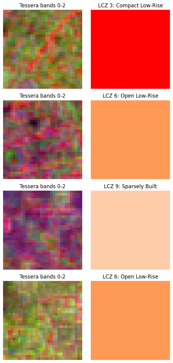
Using the UNet from train_unet.py with the small preset (depth=3, base=32).
Available: nano (2,8), small (3,32), base (3,48), medium (4,32), large (4,48).
PRESET = 'small'
depth, base_features = UNet.PRESETS[PRESET]

model = UNet(
    in_channels=IN_CHANNELS,
    num_classes=NUM_CLASSES,
    depth=depth,
    base_features=base_features,
    bottleneck_dropout=0.3,
).to(DEVICE)

print(f'Preset: {PRESET}  (depth={depth}, base={base_features})')
print(f'Parameters: {sum(p.numel() for p in model.parameters()):,}')
Preset: small (depth=3, base=32)
Parameters: 1,963,537Loss: (1 − dice_weight) × CrossEntropy + dice_weight × MulticlassDice
MulticlassDiceLoss is macro-averaged over present classes, ignoring ignore_index=-1.
ce_loss   = nn.CrossEntropyLoss()
dice_loss = MulticlassDiceLoss(NUM_CLASSES)
optimizer = optim.Adam(model.parameters(), lr=1e-3, weight_decay=1e-4)
scheduler = optim.lr_scheduler.CosineAnnealingLR(optimizer, T_max=EPOCHS)

def combined_loss(logits, masks):
    ce   = ce_loss(logits, masks)
    dice = dice_loss(logits, masks)
    return (1.0 - DICE_WEIGHT) * ce + DICE_WEIGHT * dice, ce, dice

for epoch in range(1, EPOCHS + 1):
    # --- train ---
    model.train()
    t_loss = t_ce = t_dice = 0.0
    for images, masks in train_loader:
        images, masks = images.to(DEVICE), masks.to(DEVICE)
        optimizer.zero_grad()
        loss, ce, dice = combined_loss(model(images), masks)
        loss.backward()
        optimizer.step()
        t_loss += loss.item(); t_ce += ce.item(); t_dice += dice.item()
    n = len(train_loader)
    t_loss /= n; t_ce /= n; t_dice /= n
    scheduler.step()

    # --- val ---
    model.eval()
    v_loss = v_ce = v_dice = 0.0
    correct = total = 0
    with torch.no_grad():
        for images, masks in val_loader:
            images, masks = images.to(DEVICE), masks.to(DEVICE)
            logits = model(images)
            loss, ce, dice = combined_loss(logits, masks)
            v_loss += loss.item(); v_ce += ce.item(); v_dice += dice.item()
            preds = logits.argmax(dim=1)
            correct += (preds == masks).sum().item()
            total   += masks.numel()
    m = len(val_loader)
    v_loss /= m; v_ce /= m; v_dice /= m

    print(
        f'Epoch {epoch:02d}/{EPOCHS}'
        f'  train={t_loss:.4f} (ce={t_ce:.4f} dice={t_dice:.4f})'
        f'  val={v_loss:.4f} (ce={v_ce:.4f} dice={v_dice:.4f})'
        f'  val_acc={correct/total:.4f}'
    )
Epoch 01/5 train=0.8171 (ce=1.1119 dice=0.5223) val=0.4026 (ce=0.5040 dice=0.3013) val_acc=0.8433
Epoch 02/5 train=0.4562 (ce=0.6010 dice=0.3114) val=0.3021 (ce=0.3795 dice=0.2247) val_acc=0.8929
Epoch 03/5 train=0.3594 (ce=0.4779 dice=0.2409) val=0.2186 (ce=0.2721 dice=0.1650) val_acc=0.9143
Epoch 04/5 train=0.2891 (ce=0.3783 dice=0.1999) val=0.1821 (ce=0.2249 dice=0.1394) val_acc=0.9303
Epoch 05/5 train=0.2536 (ce=0.3308 dice=0.1763) val=0.1641 (ce=0.2019 dice=0.1264) val_acc=0.9421model.eval()
images, masks = next(iter(val_loader))
with torch.no_grad():
preds = model(images.to(DEVICE)).argmax(dim=1).cpu()
n_show = 4
fig, axes = plt.subplots(n_show, 3, figsize=(9, 3 * n_show))
for i in range(n_show):
img = images[i, :3].permute(1, 2, 0).numpy()
img = (img - img.min()) / (img.max() - img.min() + 1e-8)
gt_cls = masks[i, 0, 0].item() + 1
pred_cls = preds[i].flatten().mode().values.item() + 1
axes[i, 0].imshow(img)
axes[i, 0].set_title('Bands 0-2')
axes[i, 0].axis('off')
axes[i, 1].imshow(masks[i].numpy(), cmap=lcz_cmap, norm=lcz_norm)
axes[i, 1].set_title(f'GT: LCZ {gt_cls} ({lcz_dict[gt_cls]["alt_code"]})')
axes[i, 1].axis('off')
axes[i, 2].imshow(preds[i].numpy(), cmap=lcz_cmap, norm=lcz_norm)
axes[i, 2].set_title(f'Pred: LCZ {pred_cls} ({lcz_dict[pred_cls]["alt_code"]})')
axes[i, 2].axis('off')
plt.tight_layout()
plt.show()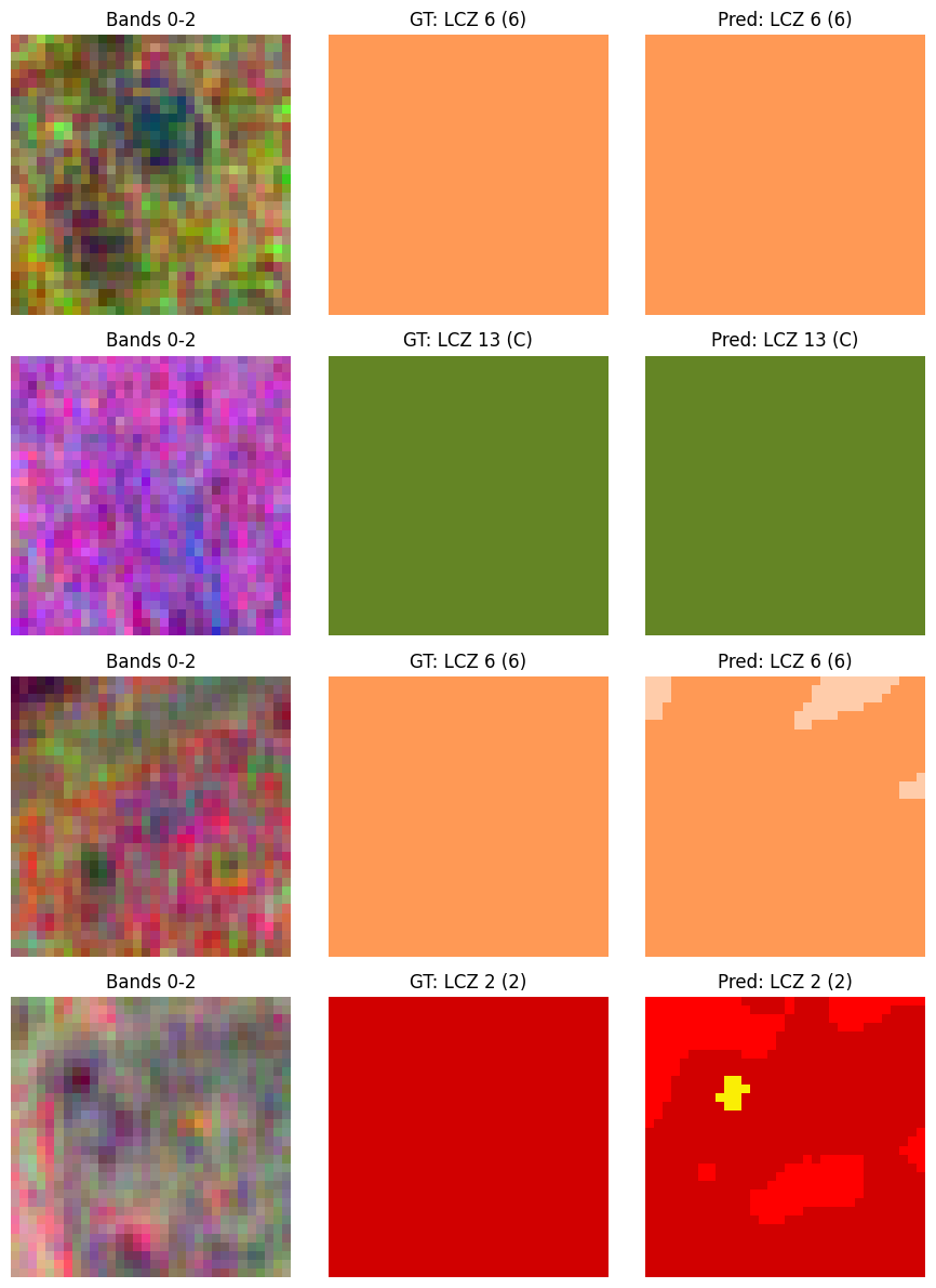
Use torchgeo’s RasterDataset + GridGeoSampler to tile the entire label area,
run inference on each patch, then mosaic the results into a single prediction map.
from torchgeo.datasets import RasterDataset
from torchgeo.samplers import GridGeoSampler, Units
from torchgeo.datasets.utils import stack_samples

class TesseraDataset(RasterDataset):
    filename_glob = '*.tif'

tessera_ds = TesseraDataset(paths=TIF_DIR)
print(f'Tiles: {len(tessera_ds.index)}  CRS: {tessera_ds.crs}  res: {tessera_ds.res}')

# Restrict inference to the So2Sat label area
roi_minx, roi_miny, roi_maxx, roi_maxy = gdf.total_bounds
roi = shapely_box(roi_minx, roi_miny, roi_maxx, roi_maxy)

pred_sampler = GridGeoSampler(
    tessera_ds, size=PATCH_SIZE, stride=PATCH_SIZE, roi=roi, units=Units.PIXELS
)
print(f'Inference patches: {len(pred_sampler)}')
Tiles: 56 CRS: PROJCS["WGS 84 / UTM zone 37S",GEOGCS["WGS 84",DATUM["WGS_1984",SPHEROID["WGS 84",6378137,298.257223563,AUTHORITY["EPSG","7030"]],AUTHORITY["EPSG","6326"]],PRIMEM["Greenwich",0,AUTHORITY["EPSG","8901"]],UNIT["degree",0.0174532925199433,AUTHORITY["EPSG","9122"]],AUTHORITY["EPSG","4326"]],PROJECTION["Transverse_Mercator"],PARAMETER["latitude_of_origin",0],PARAMETER["central_meridian",39],PARAMETER["scale_factor",0.9996],PARAMETER["false_easting",500000],PARAMETER["false_northing",10000000],UNIT["metre",1,AUTHORITY["EPSG","9001"]],AXIS["Easting",EAST],AXIS["Northing",NORTH],AUTHORITY["EPSG","32737"]] res: (10.0, 10.0)
Inference patches: 8008def pred_collate(batch):
# stack_samples handles stacking tensor fields; 'bounds' is a (9,) tensor per sample
# -> stacked to (N, 9): [minx, maxx, xstep, miny, maxy, ystep, tmin, tmax, tstep]
return stack_samples(batch)
pred_loader = DataLoader(
tessera_ds, batch_size=BATCH_SIZE, sampler=pred_sampler,
num_workers=4, collate_fn=pred_collate,
)
# Run inference, collect (pred_patch, minx, miny, maxx, maxy) per patch
model.eval()
patch_results = [] # list of (H, W) arrays with their spatial bbox
res = tessera_ds.res[0] # scalar pixel size in CRS units
with torch.no_grad():
for batch in pred_loader:
logits = model(batch['image'].float().to(DEVICE))
preds = logits.argmax(dim=1).cpu().numpy() # (N, H, W)
bounds = batch['bounds'] # (N, 9) tensor
for i in range(preds.shape[0]):
minx = float(bounds[i, 0])
maxx = float(bounds[i, 1])
miny = float(bounds[i, 3])
maxy = float(bounds[i, 4])
patch_results.append((preds[i], minx, miny, maxx, maxy))
print(f'Collected {len(patch_results)} patches')Collected 8008 patches# Assemble patches into a full raster
all_minx = min(p[1] for p in patch_results)
all_miny = min(p[2] for p in patch_results)
all_maxx = max(p[3] for p in patch_results)
all_maxy = max(p[4] for p in patch_results)
out_w = int(round((all_maxx - all_minx) / res))
out_h = int(round((all_maxy - all_miny) / res))
raster = np.full((out_h, out_w), fill_value=-1, dtype=np.int16)
for pred, minx, miny, maxx, maxy in patch_results:
col = int(round((minx - all_minx) / res))
row = int(round((all_maxy - maxy) / res))
ph, pw = pred.shape
raster[row:row + ph, col:col + pw] = pred
print(f'Raster: {out_h} × {out_w} px ({out_h * res / 1000:.1f} × {out_w * res / 1000:.1f} km)')
extent_utm = [all_minx, all_maxx, all_miny, all_maxy]
masked_raster = np.ma.masked_where(raster < 0, raster)
fig, axes = plt.subplots(1, 2, figsize=(16, 7))
# Left: predicted LCZ map
axes[0].imshow(masked_raster, cmap=lcz_cmap, norm=lcz_norm,
extent=extent_utm, origin='upper', interpolation='nearest')
gdf.boundary.plot(ax=axes[0], color='white', linewidth=0.3, alpha=0.4)
axes[0].set_title('Predicted LCZ (full ROI)')
axes[0].set_xlabel('Easting (m)')
axes[0].set_ylabel('Northing (m)')
# Right: ground-truth labels
gdf.plot(color=gdf[LABEL_COL].map(lambda c: lcz_dict[c]['color']), ax=axes[1], alpha=0.9)
axes[1].set_title('Ground truth (So2Sat patches)')
axes[1].set_xlabel('Easting (m)')
axes[1].set_ylabel('Northing (m)')
# Shared legend
fig.legend(handles=lcz_legend_handles(), fontsize=9, ncol=6,
loc='lower center', bbox_to_anchor=(0.5, -0.09), framealpha=0.8)
plt.tight_layout()
plt.show()Raster: 2441 × 3297 px (24.4 × 33.0 km)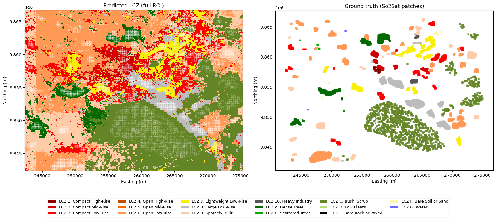
from rasterio.transform import from_bounds as rasterio_from_bounds

output_path = f'nairobi_lcz_{PRESET}_prediction.tif'

transform = rasterio_from_bounds(all_minx, all_miny, all_maxx, all_maxy, out_w, out_h)

# Write 1-indexed classes (0 = nodata) so the file is self-consistent with lcz_dict
export_raster = np.where(raster >= 0, raster + 1, 0).astype(np.uint8)

with rasterio.open(
    output_path, 'w',
    driver='GTiff',
    height=out_h, width=out_w,
    count=1,
    dtype='uint8',
    crs=TIF_CRS,
    transform=transform,
    nodata=0,
) as dst:
    dst.write(export_raster, 1)

print(f'Saved: {output_path}  ({out_h}×{out_w} px, CRS={TIF_CRS.to_epsg()})')
Saved: nairobi_lcz_small_prediction.tif (2441×3297 px, CRS=32737)